Tag: timed value

Continuation of part 1 

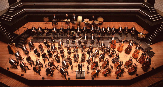
Imagine for a second that you are watching the New York Philharmonic Orchestra. As the show starts you see over 50 musicians sitting on stage and playing their musical instruments. The instruments themselves vary across the board.  There is a piano, dozens of violins, trombones, cellos, bass, etc…  As musicians begin to play, beautiful and harmonious music begins to flood the concert venue. If we stop at this juncture, we would miss an important clue that can help us time the markets with great precision.

As the music plays, a number of very important developments occur behind the scenes. To begin with, music itself is nothing more than a vibration or a wave or a cycle or an oscillation.  Each musical instrument and each player produce a range of vibrations while playing their instruments. That creates music. So a single musician will produce  a rate of vibration/oscillation that at least in technical terms is identical to the structure of the cycle. Now, having 50 musicians in our orchestra simply means that at any given second there are 50 different cycles (vibrations/waves) being created by 50 different musicians and instruments. They vary across the board and are as diverse as possible.

Yet, they all come together to create beautiful and harmonious music.  I cannot stress this enough. All 50 of the cycles (vibrations/waves)  unify  into 1 primary cycle by the time music reaches your eardrum.  No longer are you listening to 50 different vibrations, you are now listening to only one.  You are listening to the summation of these vibration, to the final result.  Finally, this end product or the summation of all of these cycles could be represented on the chart as a singular wave moving up and down over time.

What does this have to do with the stock market?

If you are to chart the final result or the final musical wave generated by the 50 musicians above it would look identical to the 2-Dimensional chart of any given stock or of the overall chart of the stock market.  It wouldn’t be identical, but it would look identical as if the music you have just heard is being tracked by the stock market charting service. This yields an important clue when it comes to the stock market cycle analysis.

Basically, there are many different cycles working in the stock market at the same time. Their range, structure, power and amplitude are as diverse as you can imagine. While some cycles last for decades and even centuries, others oscillate every few minutes. However, once we identify all of these cycles and put them all together, we end up with an exact representation of the overall stock market. When I say exact, I mean exact.

Let me repeat this. If the cycle structure is fully understood and constructed properly you can build an exact replica of the stock market. Not only for the past, but also for the future. Once the cycles are known you can predict the exact structure of all upcoming stock market moves to the point and to the day. Confirming both the fundamental and 3-DV analysis work described earlier.  

To be continued…… 

Did you enjoy this article? If so, please share our blog with your friends as we try to get traction. Gratitude!!!

 

Timing The Market With Cycles (Part 2) 

Thus far we have looked at the3-Dimensional stock market analysis as the primary tool in predicting the stock market or individual stocks in both price and time. Yet, there is another way to perform the same type of analysis.  It is called cycle work.

At the same time it is not the typical cycle work associated with the stock market. Relatively speaking cycle analysis has been around for as long as the stock market has been opened. People have been using various cycle constructs to try and predict the market.  Thus far without too much luck. Any analyst working with trying to time the markets through the use of cycle work would soon tell you that at times his cycles work perfectly fine, being able to predict the market with great accuracy and at times, they don’t work at all.  Believe it or not, there is a reason for it and that reason will be discussed in greater detail shortly.  

However, before we go any further we need to define what cycle analysis really means. In traditional sense of the word, it means studying various time cycles and then trying to apply them towards the stock market.  The simplest form of such exercise is identifying one market cycle and then trying to fit it into your market forecast. As a hypothetical example, an analyst studying NASDAQ market structure is able to determine that all stocks in the index go up for 14 trading days and then decline for 5 trading days. Then they go up for another 8 trading days and then decline for next 3 trading days. Thereafter, the cycle repeats itself indefinitely.

Of course, no such cycles exist, but it gives you an idea of how you should think about cycles. On a more complex level an analyst might put together hundreds of various cycles in order to try and predict not only the time but the value of the move.  While such cycle analysis is fairly complex, it does produce interesting and sometimes incredibly accurate results. The keyword is….sometimes.

Which begs the question, why does cycle analysis only works on limited basis?

The simple answer has to do with the 3-Dimensional analysis discussed in the previous section. The cycles do not work very well or they do break down after a certain period of time because they are being applied in the wrong medium. In this case, the 2-Dimensional chart of price moving over time. As mentioned earlier in the book, the 2-Dimensional chart construct is nothing more than a shadow of the real stock market movement. As you can imagine, no proper outcome can come from studying the shadow as opposed to studying the real move.

At the same time, when we apply cycle analysis to the 3-Dimensional construct of the market we begin to see a completely different picture. We begin to see periodicity in the cycle analysis that can be used to predict the markets with great accuracy. Not only that, but we gain a further understanding of how the markets truly works. Let me give you an example.

To be continued…… 

Did you enjoy this article? If so, please share our blog with your friends as we try to get traction. Gratitude!!! 

Timing The Market With Cycles 

Continuation of part 11

Avoid Loss Averaging: Contrary to a popular believe, it is not a good idea to buy more stock when the price declines after your purchase.  Buying more at a discounted price means you are going against the main trend and not with it. While you lower your overall purchasing price, the main issue remains. The main trend is down. Instead, you should average up when the stock price is going up. That way you are going with the trend.  

Now that we have looked at the overall rules to the profitable stock market operations, let’s take a quick look at a simple set of specific trading rules.

Rules For Trading In Stocks

RULE 1:  Buy at new high prices or old top levels.

RULE 2: Buy when prices advance above old low prices.

RULE 3: Sell when prices decline below old top levels or high prices.

RULE 4: Sell at new low price levels.  

RULE 5: Wait to buy or sell until prices CLOSE above old highs or below old lows on the daily charts. Closing price is incredibly important.

RULE 6: Use stop losses. Your capital and your profits must be protected at all times with STOP LOSSES. Implement stop losses at 1-3 points above or below your original price and at the time of the original trade.

RULE 7: Do not lose money.

In this section we have looked at 3-DV analysis, triangulation and various trading rules associated with trading the markets. By performing 3-Dimensional analysis for the DOW between 1994-today I have demonstrated without a shadow of the doubt the hidden structure within the stock market. Once that structure is fully understood (well, even before), an exact forecasts could be made. Once the analyst understands the lattice structure of the market, he can calculate it 1 year, 10 years or 100 years into the future with astonishing accuracy.

Further, we have looked at triangulation and various trading rules to minimize the risk associated with 3-Dimensional analysis.  By following all the rules described above, any stock market participant should be able to profit greatly. After all, an analyst using the work above in an appropriate fashion should know what the market will do and should act accordingly. In the next section we will look at another powerful tool to time the market with great precision. 

Did you enjoy this article? If so, please share our blog with your friends as we try to get traction. Gratitude!!!   

Stock Market And 3-Dimensional Analysis (Part 12)

Continuation of part 10

Buy At New Highs: Believe it or not, but buying at new highs is the most profitable way to make money in the market. Most people believe that they must buy at the lowest price or in the valley. That couldn’t be further from the truth. By buying at the new high you are moving with the main trend.

Sell At New Lows:  In a similar fashion, selling or selling short at the new low is the best possible position to exist the stock. It confirms that the trend has changed and gives you ability to exit your trade at a good price.  More importantly, it allows you to trade with the trend and not against it.

Never Commit To Anything:  Never attach your forecast to any fixed outcome. If you do, you will shift from the position of power to the position of fear and hope.  Opening up your trading strategy to risk and losses. Instead, remain flexible and move with the market even if your forecast indicates otherwise.

Move Stop Losses:  As the market or any given stock continue to move with the main trend you must continue to move your stop losses up or down to avoid unexpected developments and to protect your profits.  By doing so you eliminate unnecessary risk of losing money.

Don’t Be Afraid To Be Out Of The Market:  There is absolutely nothing wrong with being out of the market completely.  Sometimes for prolonged periods of time. It is better to sit on the sideline than to lose money. Particularly when the trading situation or the direction of the financial instrument you are looking at is unclear.

Don’t Wait Until The Trend Changes:  DO NOT hold your losing position in hopes of a trend change.  That is how people lose most of their money.  For instance, the bears who have been holding short positions throughout 2013 have been decimated (even though they will eventually be right).  Once again, always move with the main trend.

Get Out As Soon As You Realize You Have Made A Mistake:  Even if your in-depth research shows one thing, the market might do something completely different.   At times like this you might realize that you have made a mistake.  Do not hold your position in hope that the market will reverse itself and allow you to exit at a better price. Liquidate your position immediately.  

Always Wait For A Confirmation:  Do not establish position until and unless your work is confirmed by the market itself.  In most cases the market will do so by setting new highs or new lows. Only after receiving such a confirmation should you establish a trading position based on the main trend of the market and/or based on your own research work.

Avoid Hope & Fear: This is probably the main reason why people lose money in the stock market. They trade and/or invest on emotion rather than technical, timing or fundamental work. They hope, pray and fear instead of following exact steps.  Do not be one of these people. Never trade based on hope or fear. Follow your rules.

To Be Continued…..

Did you enjoy this article? If so, please share our blog with your friends as we try to get traction. Gratitude!!!   

Stock Market And 3-Dimensional Analysis (Part 11)

Continuation of part 9

Shortcut Two: Trading Techniques

The other way to avoid problems and/or to reduce risk when the lattice structure of the market is not yet known is to implement a strict trading regiment that would help you avoid large mistakes. By implementing strict trading rules and procedures you are able to eliminate all guess work out of the equation. In other words, while the 3-DV analysis gives you the ability to predict the markets, strict trading rules make sure you pull the trigger at the right time.

The rules below are a very simple strategy of getting in and out of stocks. Yet, it produces very powerful results while minimizing risk when you combine it with the fundamental, 3-DV and triangulation analysis  described above. First a few rules.

Avoid Low Priced Stocks:  While it is possible to make a large amount of money with these stocks, for the most part these stocks remain at low levels for a very long time.  Sometimes forever.

Avoid Slow Trading Markets or Stocks:  These are the financial instruments that are stuck in a trading range.  Do not invest in them until and unless the trend is definitely broken either to the upside or the downside.

Concentrate On Fast Moving Markets or Stocks:  This is where most money is made over the shortest period of time. Once the primary trend is identified and the 3-DV analysis work is done, buy the best stocks in the fastest moving industry.

Never Guess:  Take the guesswork (gut feeling) out of your decision making process.  Develop strict trading rules that are followed 100% of the time. While the analytical framework described above is followed, you should never guess if you got it right. Let the market and your trading rules put you in and take you out.  

Always Follow The Main Trend: You will always make money if you follow the main trend.  Either up or down. Remember, stocks are never too high to buy if the stock market is going up and they are never too low to sell if the trend is pointing down. 

Always Use Stop Losses:  I cannot overstate this enough. Always use stop losses to protect your capital. Even if you reach an advanced level in the 3-DV analysis described above, always use stop losses to make sure your work is correct.  Let the actual market prove if you are right or wrong. In the meantime, your capital base will remain save.  

To Be Continued…..

Did you enjoy this article? If so, please share our blog with your friends as we try to get traction. Gratitude!!! 

Stock Market And 3-Dimensional Analysis (Part 10)

Continuation of Part 8

Let’s take a look at the real stock market example for clarification.  Let see if we would have been able to identify point E on the chart by using triangulation. As discussed earlier, point E had 4 major 3-DVs associated with it.

1.  AE, value of 23,455. Once again and as discussed earlier, this move was the derivative (square root of 5) of 9,922 move prior to 1994. The more than typical variance of the move was caused by the growth spiral in the market.

2. CE, value of 9,810.  As shown earlier, this move was the derivative (square root of 2) of AC move of 14,100.

3. BE, value of 16,613. As discussed earlier, this move was the derivative (square root of 2) of AB move of 11,832.

4. DE, value of 8,137. From earlier discussion I have shown you that AB+BC=CD+DE=18,293. Therefore, by knowing CD, we would automatically know the value of DE (18,293-10,156)=8,137

To identify point E, well ahead of point E occurring, we would calculate where all of the 3-DVs above come together at one point. Well, a point that makes sense. After performing triangulation calculations and running the circumference of the circle for each 3-DV in question you would realize that they all come together in March of 2009.   

In other words, they all intercept each other in March of 2009, between 6,750 and 6,250 on the DOW. Further,  you would be able to get a visual confirmation that the market is indeed headed towards that same point of force you have identified through using triangulation.

In fact, this particular method has allowed me to confirm my other analysis and has allowed me to identify the March of 2009 bottom (between 6,750 and 6,250) as the highly probable turning point.  I did that in October of 2008, when the DOW was still trading between 10,000-9,000. So, as everyone was losing their minds and predicting the next Great Depression or the end of the world, an analyst familiar with 3-Dimensional analysis would know that a significant turning point is coming up in March of 2009.

Not only that, but an investor familiar with this type of analysis would simple reverse from a short position to a long position at point E to attain maximum benefit. Once the confirmation that the point E was indeed the major turning point arrives, the investor is fully aware that the next BULL move will be a prolonged one. By reallocating capital from the short side to the long side at that instance, one is able achieves maximum profitability.    

In summary, triangulation of 3-DVs allows you to find high probability turning points in 3-Dimensional space. It allows you to confirm the lattice structure if your lattice structure analysis has not advanced to the point of certainty. Further, by having multiple 3-DV’s intersect at the same point in the future, you have a fairly good idea of where the market is headed.   

(Don’t forget that this applies on all time frames).   

To Be Continued…..

Did you enjoy this article? If so, please share our blog with your friends as we try to get traction. Gratitude!!! 

Stock Market And 3-Dimensional Analysis (Part 9)

Continuation of part 7

But what if the forecast above is incorrect?

As I have mention so many times before in this book, no analyst or investor should look at any forecast in absolutely certain terms.  Until the lattice structure of the market is fully understood, there is always a possibility of being wrong. Unfortunately, understanding the lattice structure of the market is outside the scope of this book.  It is too complex and dynamic to be explained in this relatively short book. Volumes of work must be published before clarity could be obtained. Yet, any analyst willing to put in the work, should be able to determine the underlying structure.

For those unwilling to do the work there are a number of available shortcuts. They are….

Shortcut One:  3 Dimensional Space Triangulation.

Earlier in this book I have mentioned that 3-DV exist on multiple time frames. From hourly to yearly to decades to centuries.  At any given time there are hundreds of various length 3-DV tracing out market points of force (turning points). What I have found in my research over the years is that major turning points in the stock market or individual stocks are never represented by only one 3-DV. In most cases, such points are represented by a number of different 3-DV coming together at a singular turning point. Once again, these multiple 3-DV can range from hourly to centuries long.

Let me give you an example.  As you know, when 3-DV of any length moves in 3-Dimensional space they tend to trace out the circumference of a circle. The radius of a circle represents maximum reach of any given 3-DV. In other words, it represents all possible points on the two dimensional chart where the 3-DV in question can terminate its move.

Further, let’s assume that we are studying five 3-DVs from various points on the stock market chart that have similar termination points. By drawing -OR – calculating their circumferences in either 3-Dimensional space or on 2-Dimensional stock market chart, we will be able to see where those circumferences intersected.  As a rule of thumb, if we have multiple intersection at a singular point of time and price, the probability is high that such point will be a major turning point.  The probability increases further if the market is heading towards such a point.

In simple terms, triangulation allows us to figure out high probability turning points by identifying at what points multiple 3-DVs come together.  By combining this type of analysis with 3-DV lattice structure above we are able to either confirm or increase probability of a turning point.

Let’s take a look at the real stock market example for clarification.  

Did you enjoy this article? If so, please share our blog with your friends as we try to get traction. Gratitude!!! 

Stock Market And 3-Dimensional Analysis (Part 8)

Continuation of part 6

Step #2: Perform analysis of 3-DVs and its derivatives from each point.

For example, let’s take a look at point E.  At point E we can work with 4 different 3-DVs and their derivatives. They include  DE, BE, CE and AE.  Meaning, it is highly probable that EF will be equal to the four 3-DVs above and/or their derivatives.

As mentioned earlier, the 3-DV of EF today is 12,364. If we analyze the four 3-DVs above, we will soon find out that 3 different numbers closely resemble today’s value of 12,364. They are

• DE 14,094
• AE 13,542
• CE 13,873

All other 3-DVs and their derivatives either fall short or are outside the scope of our analysis. You will notice that the value AE is the closest one to our present value of 12,364. That basically means the market is not yet done moving up.  It also means that once the value AE 13,542 is reached, it is highly probable that it will mark the turning point in the stock market.

Further,  as of today the value EF consists of 2 input variables. Time Value of 7,742 trading hours and Price Value of 9,641 points.  Let’s further assume that based on our research we believe that March of 2014 will be the top of the bull market and/or the move EF.  This gives us an additional 80 trading days or 520 trading hours.  By adding 520 trading hours to 7,742 trading hours we get all necessary information to make an accurate estimate of the bull market top.

In addition,  we can estimate how much the market will move up between now and March of 2014. We simply adjust our 3-DV equation to look like this

SQRT (8,262^2 + X^2 ) = 13,542

When we solve the equation for X, the X = 10,730. This value represents the PRICE portion of the equation at the completion of the move.  With today’s PRICE value being at 9,641 this means the market is likely to go up another 1,089 points (10,730 – 9,641) between today and March of 2014.

Think about this for a second and how powerful this simple calculation is. If you got your lattice structure figured out and/or you know the next 3-DV move,  you can predict with 100% certainty exactly when the stock market will top out. Not only when, but exactly where. To the day and to the point. So, while everyone else is playing the guessing game of how long this bull market will continue, you know the answer well ahead of that turning point taking place.  You know that you must hold for another 4 months in order to realize the maximum gain and then simply reverse to short position to benefit from the upcoming bear market decline.  Amazing, isn’t it?

But what if the forecast above is incorrect?

To Be Continued…..

Did you enjoy this article? If so, please share our blog with your friends as we try to get traction. Gratitude!!!

Stock Market And 3-Dimensional Analysis (Part 7)

Continuation of part 5

7. The move AB was an exact square and continuation of another 3-DV prior to 1994 bottom. This move was a perfect square. The market moved exactly 8,296 points in exactly 8,437 trading hours. Giving us a 3-DV of 11,832.  This 3-DV was identical to the actual top set on January 14th, 2000 of 11,854. Proving, once again, how accurate this analysis can be.  

8.  Finally, the move BC was the derivative from the move AB. If you divide 11,832 by the square root of 3 you end up with a value of 6,831. With move BC having a 3-DV of 6,840, it gives us 0% variance.  As 2003 secondary bottom was approaching an analyst using 3-DV analysis would be very well aware that a turning point was coming up. Using the techniques above the analyst would be about 10 trading points away from the actual bottom.

This concludes the analysis and explanation of the 3-DV moves above.  The explanation above went over every single value and showed you how they can be used in order to predict the markets with great accuracy. Going further and by understanding the lattice structure within the market you would be able to know precise angles and directional moves of any upcoming market or individual stock moves.  For the first time attaining the ability to predict the markets in both time and price. On any time frame.  From daily resolution to decades from now.  

This section is written on November 29th,  2013 with the DOW at 16,097

If you follow my daily blog you are very well aware that my mathematical work is predicting a severe bear market between 2014 and 2017. This bear market will represent the final leg down of the bear market that started in early 2000. This brings us to point F on the chart above  and further explanation on how to predict exact turning points by using 3-DV analysis. Please keep in mind that point F represents the actual turning point in 2014 and the ushering in of the bear market leg. It hasn’t happened yet.  We are predicting the future here.  Let’s take a look.

Step #1:  Measure 3-DV from all major turning points (E, D, C, B and A)  to today’s DOW close.  They are..

• EF: 12,364
• DF: 10,610
• CF: 20,190/20,900
• BF: 24,100
• AF:  34,750

Step #2: Calculate all derivative values for the numbers above.

To Be Continued…..

Did you enjoy this article? If so, please share our blog with your friends as we try to get traction. Gratitude!!!  

Stock Market And 3-Dimensional Analysis (Part 6)

 

Continuation of part 4. 

3.  We have already mentioned this earlier in the book, but AB + Bc  and CD + DE are equal. Let’s take another look. (11,832+6,483 =  18,315)  and  (10,156 + 8,137 = 18,293). Please note that we are using 2002 actual bottom for point c instead of 2003 secondary bottom. Also note, that the variance is just 22 points over the 15 year period of time. That constitutes a margin of variance equal to just 3 trading days or a few hundred points directional move.

Also, note that if you divide 18,300  by the square root of 5 you get a value of 8,184. Which was the value of the move between 2007 top and 2009 bottom. Further, if you multiply BD of 12,815 by square root of 2 you will get a value of 18,123 which is identical to the value above.  Once again, if you know the structure of this move and lattice structure associated with the market you have the ability to identify every single turning point in the market over the last 15 years.

All you have to do at those points is to rotate your portfolio position from long to short and from short to long in order to make a killing and outperform the market by a large margin. It is as simple as that.

4.  The move CE of 9,810 and the move CD is the continuation of the move AC represented by 14,100. If you divide 14,100 by the square root of 2 you get a value of 9,970. The actual move between CE ended up being 9,810 giving us the variance of only 1.6%.  The actual move between CD ended up being 10,156 giving the variance of only 1.8%. When you combine this knowledge with the previous 3-DV already discussed you get another confirmation that March of 2009 will be a solid bottom for the stock market and that the 2007 top has been reached.

As such, when everyone is freaking out about the 2007-2009 decline and predicting the end of the world as we know it, you would know that the market will turn around in March of 2009 and begin a multiyear rally.

5. When you multiple vale AB of 11,832 by the square root of 2 you end up with a  3-DV value of 16,733. The actual move between 2000 top and 2009 bottom or the move BE was exactly 16,613. That is a variance of just 0.7%.  Again, the move AB predicted the move BE and 2009 bottom 9 years in advance. Giving you another confirmation point that March of 2009 is an exact bottom and a major turning point.

6. The move BD of 12,815 was the derivative of the move AB + Bc of 18,315.  When you divide 18,315 by the square root of 2 you end up with a 3-DV value of 12,950. This gives us a variance of just 1%.

To Be Continued….

Did you enjoy this article? If so, please share our blog with your friends as we try to get traction. Gratitude!!!